Modeling

biological processes are complicated

Model types

based on Hasenauer et al., J. Coup. Sys. and Mult. Dyn. 2015

A mathematical model is a representation of the essential aspects of a system [...] which presents knowledge of that system in usable form.

Pieter Eykhoff 1974

All models are wrong, but some are useful.

George Box 1976

The inverse problem

Parameter inference

Basic idea

e.g. an ODE model:
states: $\dot x (t, \theta) = f(t, x, \theta)$, $x(t_0, \theta) = x_0(\theta) \in \mathbb{R}^{n_x}$,
observables: $y(t, \theta) = h(x(t, \theta), \theta) \in \mathbb{R}^{n_y}$,
measurements: $\bar y_{ik} \sim \mathcal{N}(y_k(t_i,\theta), \sigma^2_{ik}(\theta) \in \mathbb{R}^{n_y}$

likelihood function: $p(D|\theta) = \prod_{ik}\frac{1}{\sqrt{2\pi}\sigma_{ik}(\theta)} \exp\left[-\frac{1}{2} \left(\frac{\bar y_{ik} - y_k(t_i,\theta)}{\sigma_{ik}(\theta)}\right)^2\right]$

objective function: $J(\theta) := - \log p(D|\theta) = \frac{1}{2}\sum_{ik}\left[\log(2\pi\sigma_{ik}^2(\theta)) + \left(\frac{\bar y_{ik} - y_k(t_i,\theta)}{\sigma_{ik}(\theta)}\right)^2\right] \overset{!}{\rightarrow}\min_{\theta\in\Theta}$

if prior knowledge is available: prior $p(\theta)$,
$J(\theta) := -\log p(D|\theta) - \log p(\theta)$

Optimization

find the best point estimate (MLE)

local vs global or multistart
derivative-free vs derivative-based
higher-order information

Hierarchical optimization

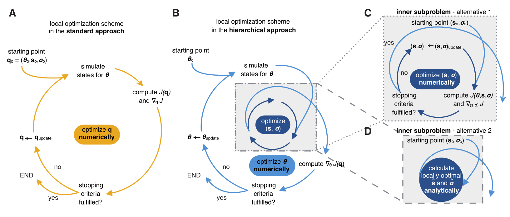Loos, Carolin, et al. "Hierarchical optimization for the efficient parametrization of ODE models." Bioinformatics 2018.

Computing gradients $\nabla J(\theta)$

$$\nabla J(\theta) = \sum_{i=1}^{n_t}\left[\frac{\partial J_i}{\partial y}(y(t_i,\theta),\theta)\color{red}{\frac{dy}{d\theta}(t_i,\theta)} + \frac{\partial J_i}{\partial \theta}(y(t_i,\theta),\theta)\right]$$

finite differences: $\delta_l J(\theta) = (J(\theta + \delta e_l) - J(\theta)) / \delta$
forward sensitivities: calculate $\frac{dx}{d\theta}$ via additional ODEs
adjoint sensitivities: circumvent $\frac{dx}{d\theta}$ via a cheaper adjoint state

finite differences

$$\delta^{h}_lJ(\theta) = \frac{J(\theta + \frac 1 2h\cdot e_l) - J(\theta - \frac 1 2h\cdot e_l)}{h}$$

inefficient: $O(n_xn_\theta)$
numerically unstable

forward sensitivities

$$\nabla J(\theta) = \sum_{i=1}^{n_t}\left[\frac{\partial J_i}{\partial y}(y(t_i,\theta),\theta)\frac{dy}{d\theta}(t_i,\theta) + \frac{\partial J_i}{\partial \theta}(y(t_i,\theta),\theta)\right]$$ where, with $s^x = \frac{dx}{d\theta}$, the extended ODE
$\dot x = f, x(0) = x_0$,
$\dot s^x_l = \frac{\partial f}{\partial x}s^x_l + \frac{\partial f}{\partial \theta_l}, s^x_l(0) = \frac{\partial x_0}{\partial\theta_l}, l=1,\ldots,n_\theta$
allows us to calculate $\frac{dy}{d\theta}$

inefficient: $O(n_xn_\theta)$
numerically robust
can exploit ODE structure

adjoint sensitivities

Idea: introduce an adjoint state $p\in\mathbb{R}^{n_x}$ such that $$\nabla J(\theta) = \sum_{i=1}^{n_t}\left[\frac{\partial J_i}{\partial\theta} + \frac{\partial J_i}{\partial y}\frac{\partial h}{\partial\theta}\right] - p(t_0)^T\frac{d x_0}{d\theta}(\theta) - \int_{t_0}^{t_{n_t}}p^T\frac{\partial f}{\partial\theta}d\tau$$ without the annoying $\frac{dx}{d\theta}$!
$p$ is uniquely defined by the backward ODE $$\dot p = -\frac{\partial f}{\partial x}^Tp\quad\text{with initial condition}\quad p(t_{i}) = \lim_{t\searrow t_{i}}p(t) - \left(\frac{\partial J_{i}}{\partial y}\frac{\partial h}{\partial x}\right)^T$$

in practice nearly $O(n_x)$ (2 ODEs and a simple quadrature)
more involved implementation
no least-squares optimizers applicable

github.com/amici-dev/amici
high-performance ODE simulation and sensitivity calculation

Uncertainty analysis

Profile likelihoods

profile likelihoods defined as $\text{PL}_{g(\theta)}(c) = \max_{\theta\in g^{-1}(c)}p(D|\theta)$
confidence intervals derived from likelihood-ratio tests
profiles calculated via optimization / integration / local approximation

Bayesian inference

Posterior analysis

Often, we are interested in integrals of the posterior, e.g.

Posterior mean of a parameter: $\mathbb{E}(\theta|D) = \int \theta p(\theta|D)d\theta$
Posterior variance (uncertainty): $\mathbb{V}(\theta|D) = \mathbb{E}(\theta^2|D) - \mathbb{E}(\theta|D)^2$
Credible intervals: $\mathbb{P}(\theta\in[l,u]|D) = \int_l^u p(\theta|D)d\theta$
Marginals: $p(\theta_1|D) = \int p(\theta|D)d\theta_2\cdots d\theta_n$

Monte-Carlo sampling can be used to approximate expectations: $$\mathbb{E}(f(\theta)|D) \overset{n\rightarrow\infty}{\approx} \frac{1}{n}\sum_if(\theta_i)$$ with $\theta_i \overset{\text{iid}}{\sim} p(\theta|D)$.

How to sample from a distribution?

Simple distributions: CDF inversion $F_{p(\theta|D)}^{-1}(U[0,1])$
Rejection sampling: $\theta\sim q(\theta)$, accept if $U[0,1] < p(\theta|D)/(Mq(\theta))$
Importance sampling: $\mathbb{E}_{p(\theta|D)}(f) = \int f(\theta)\frac{p(\theta|D)}{q(\theta)}q(\theta)d\theta$

does not really scale well to high-dimensional distributions ...

Markov-Chain Monte-Carlo (MCMC)

idea: instead of randomly drawing iid samples, evolve samples via small perturbations to what was already observed

until chain long enough:

propose $\theta \sim q(\theta|\theta_i)$
if $U[0,1] < \min\left(1,\frac{p(\theta|D)q(\theta|\theta_i)}{p(\theta_i|D)q(\theta_i|\theta)}\right)$, then $\theta_{i+1}=\theta$, else $\theta_{i+1} = \theta_i$

Markov-Chain Monte-Carlo (MCMC)

More refined updates (Hamiltonian Monte-Carlo, NUTS, ...)
Adapt to problem structure
Parallel Tempering

Further topics

Outlier control
Model selection
Ordinal data
Mixed effects
Standards
Residual analysis
Structural identifiability
...

github.com/icb-dcm/pypesto
parameter estimation toolbox

optimization, profiles, sampling
own implementations and interfaces to popular tools
high-performance computing parallelization
model selection, visualization, ...

github.com/petab-dev/petab
data format for specifying parameter estimation problems

Literature

Fröhlich, Fabian, et al. "AMICI: High-Performance Sensitivity Analysis for Large Ordinary Differential Equation Models." arXiv preprint arXiv:2012.09122 (2020).
Fröhlich, Fabian, Carolin Loos, and Jan Hasenauer. "Scalable inference of ordinary differential equation models of biochemical processes." Gene Regulatory Networks (2019): 385-422.
Raue, Andreas, et al. "Lessons learned from quantitative dynamical modeling in systems biology." PLoS ONE, 8(9):e74335, 2013.
Ballnus, Benjamin, et al. "Comprehensive benchmarking of Markov chain Monte Carlo methods for dynamical systems." BMC Systems Biology, 11(63), 2017.

Likelihood-free inference

Likelihood-free Bayesian inference

common optimization and sampling methods (e.g. MCMC) require the (unnormalized) likelihood
can happen: numerical evaluation infeasible
... but still possible to simulate data $y\sim\pi(y|\theta)$

Example: Modeling tumor growth

based on Jagiella et al., Cell Systems 2017 Tumor gif

cells modeled as interacting stochastic agents, dynamics of extracellular substances by PDEs
simulate up to 10⁶ cells
10s - 1h for one forward simulation
7-18 parameters

What we tried

multi-start local methods
- deterministic gradient descent
- stochastic gradient descent
- Bayesian optimization
global methods
- simulated annealing
- > 20 particle methods
- enhanced scatter search

Failed	Worked
multi-start local methods deterministic gradient descent Levenberg-Marquardt interior-point trust-region stochastic gradient descent Bayesian optimization global methods simulated annealing > 20 particle methods enhanced scatter search	---

How to infer parameters for complex stochastic models?

ABC

Approximate Bayesian Computation

Rejection ABC

With distance $d$, threshold $\varepsilon>0$, summary statistics $s$:

until $N$ acceptances:

sample $\theta\sim g(\theta)$
simulate data $y\sim\pi(y|\theta)$
accept $\theta$ if $d(s(y), s(y_\text{obs}))\leq\varepsilon$

A "derivation"

Rejection sampling

Background: Want to sample from $f$, but can only sample from $g \gg f$.

until $N$ acceptances:

sample $\theta\sim g(\theta)$
accept $\theta$ with probability $\propto \frac{f(\theta)}{g(\theta)}$

Accepted $\theta$ are independent samples from $f(\theta)$.
Let $f=\pi(\theta|y_\text{obs}), g=\pi(\theta) \Rightarrow \frac{\pi(\theta|y_\text{obs})}{\pi(\theta)} \propto \pi(y_\text{obs}|\theta)$

not available
idea: circumvent likelihood evaluation by simulating data and matching them to the observed data

Likelihood-free rejection sampling

until $N$ acceptances:

sample $\theta\sim \pi(\theta)$
simulate data $y\sim\pi(y|\theta)$
accept $\theta$ if $y=y_\text{obs}$

Acceptance probability: $\mathbb{P}[y_\text{obs}]$
can be small in particular for continuous data
idea: accept simulations that are similar to $y_\text{obs}$

Rejection ABC

With distance $d$, threshold $\varepsilon>0$:

until $N$ acceptances:

sample $\theta\sim \pi(\theta)$
simulate data $y\sim\pi(y|\theta)$
accept $\theta$ if $d(y, y_\text{obs})\leq\varepsilon$

curse of dimensionality: if the data are too high-dimensional, the probability of simulating similar data sets is small
idea: create an informative lower-dimensional representation via summary statistics
ideally minimal sufficient statistics

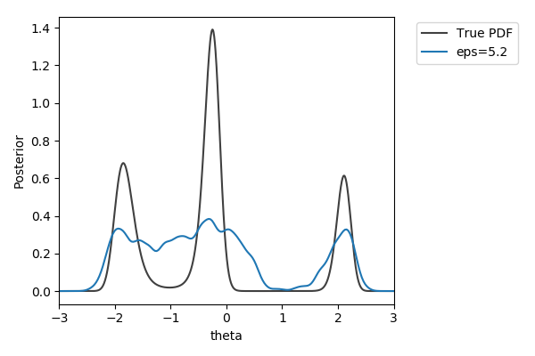
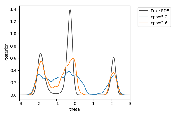
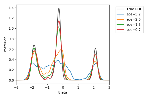
Toy example

$y\sim\mathcal{N}(2(\theta-2)\theta(\theta+2), 1+\theta^2)$, $y_\text{obs}=2$
$\pi(\theta) = U[-3,3]$
$d=|{\cdot}|_1$
$N=1000$ acceptances

Approximate Bayesian Posterior

We want: \[\pi(\theta|y_\text{obs}) \propto \color{red}{p(y_\text{obs}|\theta)}\pi(\theta)\]

We get: \[\pi_{ABC}(\theta|s(y_\text{obs})) \propto \color{red}{\int I(\{d(s(y), s(y_\text{obs})) \leq \varepsilon\})p(y|\theta)\operatorname{dy}}\pi(\theta) \approx \frac{1}{N} \sum_{i=1}^N\delta_{\theta^{(i)}}(\theta)\] with distance $d$, threshold $\varepsilon>0$, and summary statistics $s$

Sources of approximation errors in ABC

model error (as for every model of reality)
Monte-Carlo error (as for sampling in general)
summary statistics
epsilon threshold

Far better an approximate answer to the right question, which is often vague, than an exact answer to the wrong question, which can always be made precise.

John Tukey 1962

Efficient samplers

Rejection ABC, the basic ABC algorithm, can be inefficient due to repeatedly sampling from the prior
smaller $\varepsilon$ leads to lower acceptance rates
many (likelihood-based) algorithms like IS, MCMC, SMC, SA have ABC-fied versions

github.com/icb-dcm/pyabc
Klinger et al., Bioinformatics 2018

Easy to use

                
# define problem
abc = pyabc.ABCSMC(model, prior, distance)

# pass data
abc.new(database, observation)

# run it
abc.run()

Parallel backends: 1 to 1,000s cores

Parallelization strategies

Klinger et al., CMSB Proceedings 2017 Parallelization strategies

Example: Tumor growth model

based on Jagiella et al., Cell Systems 2017

Define summary statistics

400 cores
2 days
1.8e6 simulations

ABC worked where many other methods had failed.

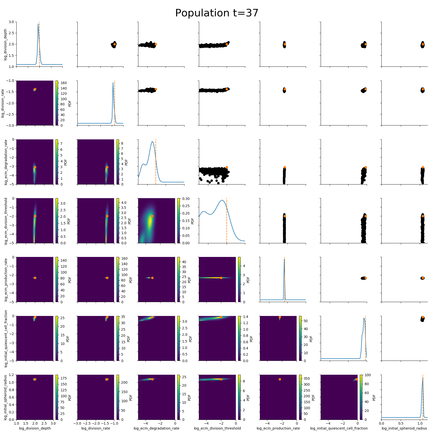
ABC worked where many other methods had failed.

Uncertainty-aware predictions, easy data integration.

Algorithmic details

Adaptive population sizes

Klinger et al., CMSB Proceedings 2017 Adaptive population sizes

idea: adapt population size trying to match a target accuracy

Self-tuning distance functions

based on Prangle, Bayesian Analysis 2015
Adaptive distances

Measurement noise

Schälte et al., Bioinformatics 2020
How to efficiently account for measurement noise in ABC? Measurement noise methods

Further challenges

Summary statistics calculation
Epsilon thresholds
Model selection
Early rejection
...

And ...

...

Joint initiative to perform inference for multi-cellular models

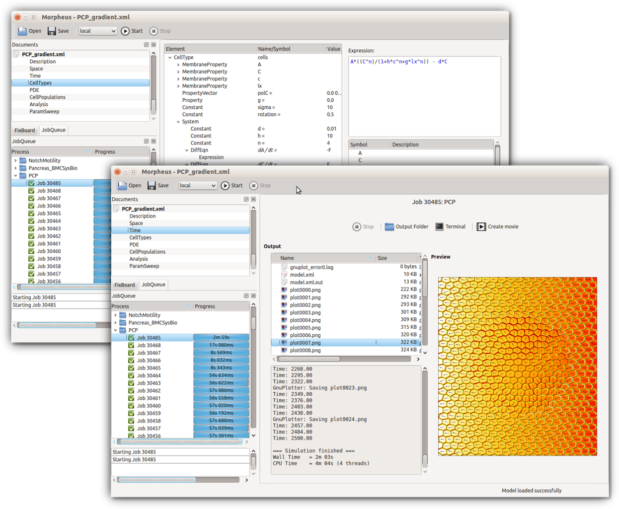
Morpheus toolbox: Staruß et al., Bioinformatics 2014

Literature

Sisson, Scott A., Yanan Fan, and Mark Beaumont, eds. "Handbook of approximate Bayesian computation." CRC Press, 2018.
Beaumont, Mark A. "Approximate Bayesian computation in evolution and ecology." Annual review of ecology, evolution, and systematics 41 (2010): 379-406.
Martin, Gael M., David T. Frazier, and Christian P. Robert. "Computing Bayes: Bayesian Computation from 1763 to the 21st Century." arXiv preprint arXiv:2004.06425 (2020).

Acknowledgments

Thanks to: Jan Hasenauer, Emad Alamoudi, Jakob Vanhoefer, the whole lab, ...

Modeling

Model types

The inverse problem

Parameter inference

Basic idea

Basic idea

Optimization

Hierarchical optimization

Computing gradients $\nabla J(\theta)$

finite differences

forward sensitivities

adjoint sensitivities

Uncertainty analysis

Profile likelihoods

Bayesian inference

Posterior analysis

How to sample from a distribution?

Markov-Chain Monte-Carlo (MCMC)

Markov-Chain Monte-Carlo (MCMC)

Further topics

Literature

Likelihood-free inference

Likelihood-free Bayesian inference

Example: Modeling tumor growth

What we tried

Failed

Worked

How to infer parameters for complex stochastic models?

ABC

Rejection ABC

A "derivation"

Rejection sampling

Likelihood-free rejection sampling

Rejection ABC

Toy example

Approximate Bayesian Posterior

Sources of approximation errors in ABC

Efficient samplers

Easy to use

Parallel backends: 1 to 1,000s cores

Parallelization strategies

Example: Tumor growth model

Define summary statistics

Algorithmic details

Adaptive population sizes

Self-tuning distance functions

Measurement noise

Further challenges

And ...

...

Literature

Acknowledgments

Thanks! Questions?